── Attaching core tidyverse packages ──────────────────────── tidyverse 2.0.0 ──
✔ dplyr     1.1.4     ✔ readr     2.1.4
✔ forcats   1.0.0     ✔ stringr   1.5.1
✔ ggplot2   3.4.4     ✔ tibble    3.2.1
✔ lubridate 1.9.3     ✔ tidyr     1.3.0
✔ purrr     1.0.2
── Conflicts ────────────────────────────────────────── tidyverse_conflicts() ──
✖ dplyr::filter() masks stats::filter()
✖ dplyr::lag()    masks stats::lag()
ℹ Use the conflicted package (<http://conflicted.r-lib.org/>) to force all conflicts to become errors
Day Two:
Pipe(s)
~20 min
Overview
Questions
- What is a
pipe,and how it works? - Which pipes should we know and care about?
Lesson Objectives
To be able to
- Use the R native pipe (
|>) to concatenate functions, knowing that the magrittr one (%\>%) has similar behavior.
Pipes
…, and then…, and then…, and then …, …
Setup overview
We adopted the Tidyverse ecosystem during the course using the tidyverse R package.
Tip
-
pkg::fun()explicitly tells R the package to look for the function. - If multiple packages have functions with the same name, and if the package is not indicated explicitly in the call, the last attached one (i.e.,
?libraryed) has the priority (i.e., it masks the others). - Using
pkg::fun()instead offun(), you are sure about the function R calls.
Your turn
- Connect to our pad(https://bit.ly/ubep-rws-pad-ed3)
- Put an
Xnext to the correct answer, under section 2.3 Ex10 in the pad.
If you attach only the tidyverse package in a new R session, and you call filter(), which function are you calling?
-
stats::filter(). -
dplyr::filter(). - An error due to ambiguity.
- I don’t know what
stats::filter()ordplyr::filter()means in R. - Other (please specify)
02:00
Tidyverse convention
One of the advantages of the Tidyverse is that common standards make everything easier to remember, understand (e.g., when reading the code for self or other people), and apply.
Important
- Functions are verbs (they do something)
- argument and objects are nouns (they are something)
- Functions first argument is always data (tibble/data frames)
- Output is always data.
- Output is always the same type of data (whatever input or option is provided)
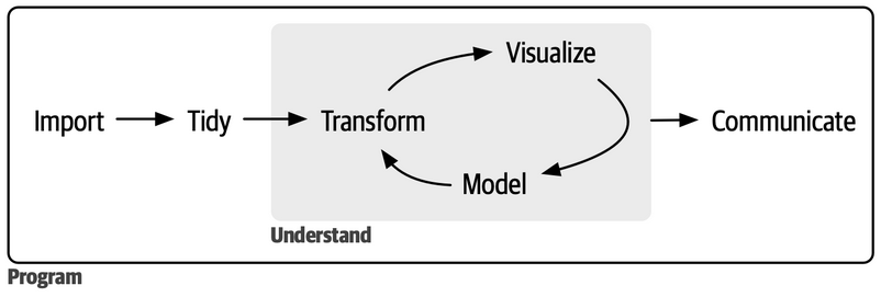
Data analyses: a sequence of actions
Import: define a path, and then… read it, and then… initial fixes (e.g., removing empty rows or columns)
Tidying: take the data, and then… separate merged information, and then…, …, and then… reshape the data to tidy them
Transforming: take the data, and then… mutate some variables accordingly to desiderata (e.g., making factors, converting dates, or cleaning text, and then… filter unwanted observations for the current study.
Visualize: take the data, and then… select what to plot, and then… define how to plot, and then… restyle accordingly to desiderata, and then… save it.
Analyse: take the data, and then… reshape it accordingly to the model requirements, and then… fit the model, and then… summarize the model, and then… plot the results

Mental exercise
Suppose you have the following functions:
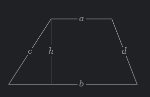
Pretend that it is a difficult problem, and you want to use those functions only to find a trapezoid area with the following data already defined in your R session:
Your Turn
You can type your answer on sec 2.3 Ex.11 in the pad.
Area = \(\frac{a+b}{2}h\)

02:00
Overwrite the result [side-by-side]
What if we need to debug this code? If we make mistakes, we’ll need to re-run the complete pipeline from the beginning!
It is hard to follow what is change each line considering that we repeated
res(that is the name of our final result) six time!
Change name every time can surely solve 2. Let see.
Create middle objects [side-by-side]
[1] 10- We didn’t repeat names, but now we have a lot of unuseful names (and objects!) defined in our workspace.
We must think of meaningful (unuseful!) names for all the intermediate objects, because we surely want to avoid situations like the following one
[1] 10Which takes the worst of both, adding the difficult in debugging and correcting all the numbers in intermediate changes happened; or, worst, starting having non-sequential numbered variable names!
So we can compose functions one inside other to get the resutl directly! Let see
Compose function calls [side-by-side]
- Quite unreadable and extremely difficult to follow; mainly because each argument is at a increasing distance from its function names (e.g.,
multiply_byis the first name appearing, and its second argumenthis the last one!)
We could improve readability by indenting our code (which is surely a good thing to do)
But, it remain quite difficult to understand what the function does; at least, it is not immediate natural!
So that are the reasons wy we need a tool, and that is the pipe. Let’s have a look at it.
Use pipes [side-by-side]
In it simpler definition the pipe (which now a native symbol in R |>) is an operator that takes the result of whatever is evaluated in its left and use it as the first input of the function call at its right (that must be a proper function call, with at least one argument)
Tip
In math point of view, pipe transforms \(f(x,\ y)\) into \(x\ |> f(y)\). So that we can restructure \(f(g(x))\) as \(g(x)\ |> f()\).
Tip
Try to read the pipe as “and than…”
- Every argument is exactly next to its function call
- We create the result object only
- We can naturally read what the code do: “take a, and then… add b, and then… divide the result by two, and then… multiply the result by h”; and that’s it, the spelled formula of trapezoid areas!
Anonymous functions (Optional)
Important
Native pipe operator |> and anonymous functions were both introduced in R 4.1.0.
Anonymous functions are… functions without a name! They are often used for short, throwaway operations.
- Syntax (definition):
\(x) { ... }wherexis the argument and{ ... }is the function body. - Syntax (call):
(\(x) { ... })(val)wherevalis the value to pass to the function.
Important
The right side of the pipe must be a function call, and not a function definition! So, we need to enclose the function definition in parentheses () to make us able to call it immediately addin
Tip
Anonymous functions are often used with pipes, because we can define a function directly in the pipe, and use it immediately.
{magrittr} vs native [optional]
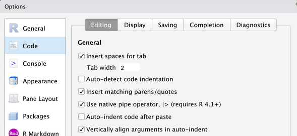
Pipes in R first appear with the magrittr package in 2014 as %>%, and it has been part of the tidyverse since that time. Now it still in the tidyverse, and still the default in RStudio IDE keyboard shortcut CTRL/CMD + SHIFT + M.
Now, Tidyverse team suggest to switch to the native pipe, appearing in R 4.0.1 in 2021.1
Tip
Change the RStudio default shortcut CTRL/CMD + SHIFT + M to use the native pipe.

Your turn (main: C; bk1: A; bk2: B)
Your turn
Connect to our pad(https://bit.ly/ubep-rws-pad-ed3) (Ex. 12)
Connect to Day 2 project on our RStudio cloud (https://bit.ly/ubep-rws-rstudio)
Imagine we have a dataset representing the daily number of new infection cases reported in a specific area over a week. Unfortunately, there was a day when data couldn’t be collected due to a system malfunction, resulting in a missing value. Our goal is to calculate the average (2 significant digits) day-to-day fluctuation in the number of new cases reported over the week.This measure can help public health officials understand the volatility in the spread of the infection and potentially identify any unusual spikes or drops in case numbers.
Open the script
07-pipe.R, and reformat the code using the native pipe the code.In the pad, under section
2.3 - Ex.12report your preference putting an X next to your selection.
You can solve the problem with the following code:
[1] 28.3315:00
My turn
YOU: Connect to our pad (https://bit.ly/ubep-rws-pad-ed3) and write there questions & doubts (and if I am too slow or too fast)
ME: Connect to the Day-2 project in RStudio cloud (https://bit.ly/ubep-rws-rstudio): script 07-pipe.R
Acknowledgment
To create the current lesson, we explored, used, and adapted content from the following resources:
- Carpentrie’s Programming with R course material.
- Carpentrie’s R for Reproducible Scientific Analysis course material.
- Hadley Wickham’s Advanced R - (2e)
- Hadley Wickham’s R for Data Science
- Hadley Wickham’s R for Data Science (2e)
The slides are made using Posit’s Quarto open-source scientific and technical publishing system powered in R by Yihui Xie’s Kintr.
Additional resources
License
This work by Corrado Lanera, Ileana Baldi, and Dario Gregori is licensed under CC BY 4.0

UBEP’s R training for supervisors